The first thing most professional portfolio managers do before making any trade decisions is assess current market conditions. That is why they get to the office well before the markets open to digest all new information and its impact on current prices. They also typically have access to analytic tools to process all this information. Ripsaw® provides robust wealth management tools that capture what the stock and bond markets are offering at this instant for future expected return and risk dimensions.
Our objective is to gather and provide information that will improve the performance of your investment decisions. For example, we would certainly like to know how risky the stock market is going forward? What is the current compensation for moving cash into the stock market now? How risky are long-term government bonds, investment grade corporate bonds, high yield corporate bonds, and mortgage-backed securities today? What is the current compensation for taking on risk in each of these sectors? How much risk reduction (diversification) will I get from allocating wealth across these sectors?
While researchers use historical returns and statistics to answer some of these questions, we need to update this information with the market’s current view of the future impounded in today’s prices. Historical volatilities tell us something about past risk. Although we can look at historical sub-periods that have similar economic circumstances as today, it is impossible to find an exact match for the current environment. During the financial crisis of 2008, new announcements came to the marketplace every day. The government takeover of Fannie Mae and Freddie Mac, Lehman Brothers failure, and Federal Reserve policy changes were all partially anticipated in market prices before these events occurred. Even use of recent historical data is behind the rapid flow of relevant information. Using historical data from months before February of 2020, had trivial, if any, information about the pandemic that ensued. Hence, we need to take advantage of those financial instruments that tell us how the market is interpreting the information flow as it occurs for future risk and expected return. This can all be easily found in the Ripsaw® Market Analysis toolset.
The two most useful sources of forward-looking information are the US Treasury Yield Curve and the CBOE Volatility Index® (VIX®). Comparing Treasury yields of different maturities provides valuable information concerning the market’s view of the path of future yields (forward rates) and expected inflation. VIX® is the implied volatility from option prices on the S&P 500 stock portfolio. Option prices are a function of known contract terms and the expected volatility over the life of the contract. VIX® employs price as an input to solve for the implied volatility among several option contracts on the S&P 500 to create its index. Therefore, VIX® is a measure of the future risk of investing in the S&P 500 stock portfolio with all knowledge of the past and instant updates on assessments about future risk imbedded in its price. With these forward-looking pieces of information, Ripsaw® updates the expected return, volatility, and correlations among investment opportunities with a more complete view of expectations than history alone.
The market price of an investment is a complex weighted average of all participating investors with heterogeneous views of the expected future cash flows and its risk dimensions weighted by their respective degrees of risk aversion and dollars of investment. Although each investor has their own opinion on a particular investment, we can say that the observed market price of an investment is the present value of the “consensus” expected cash flows over the life of the investment discounted back to the present at their “consensus” risk-adjusted discount rates.
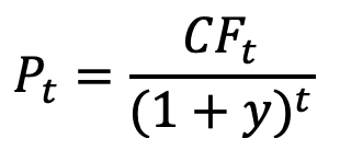
Always be thinking about the General Valuation Equation. The current price of an investment, P0, is equal to the present value of all future expected cash flows in the numerators, Xt, from time t = 1, … to N, discounted back to time 0 at the per-period sequence of risk-adjusted discount rates in the denominators, Rt.
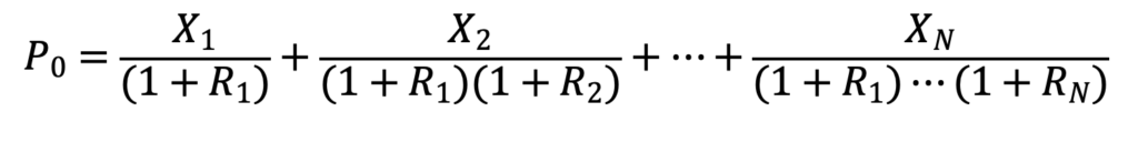
Where Rt = Riskless Ratet + Risk Premiumt.
For a US Treasury bond, N is the time to maturity, Xt represents all the known with certainty coupon payments prior to maturity and XN contains the last certain coupon and principal payment. All Rs are equal to the yield to maturity. For risky bonds, all the coupon and principal payments are only promises, not for certain. In these cases, all Xts are expected coupons and the expected principal payment at maturity. The discount rates include a risk premium that investors charge to compensate for all possible instances (probability distribution) of default and recovery rates.
Equity ownership (stock holdings) has no maturity date (N is infinite). All Xts are expected cash flows to stockholders where the discount rates include a risk premium that investors charge to compensate for all possible deviations from expected cash flows (probability distribution) due to unanticipated changes in the economic environment, management effectiveness, product competitiveness, etc.
The US Treasury Yield Curve has forward-looking information for the nominal Riskless Rate and VIX® has forward-looking information concerning the Risk Premium in the risk-adjusted discount rates. If either or both discount rate components increase, price declines. If either or both components decline, price increases. However, if Treasury yields and VIX® move in opposite directions, the dominate impact will determine the price change, but the magnitude of the price change will be mitigated by the other.
Note that all the emphasis in the General Valuation Equation is on future cash flows and discount rates. Not the past! Historical information is useful to the extent that it helps market participants assess the probabilities of future outcomes. Using only historical data is like trying to drive a car forward by only looking in the rearview mirror. Not good!
As new information is impounded in price, we have the US Treasury Yield Curve and VIX® for assessing the market’s interpretation of the risk-adjusted discount rates. But those assessments are not independent of the expected future cash flows to investors in the numerator. While the uncertainty about those expected cash flows is incorporated in the risk premium, the implications for the level and path of expected cash flows are determined by the market consensus. Therefore, it is important for investors to analyze the new information effect on all three components of valuation.
Inputs to construct or revise a portfolio today for a specific investment horizon includes assessments of the expected future return and risk of each security as well as all the pairwise correlations among securities. The goal is a preferred allocation of wealth among all securities in all accounts consistent with your investment objectives.
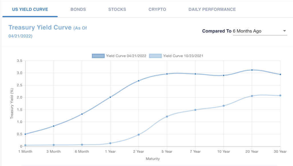
The Treasury Yield Curve provides current nominal U.S. government borrowing rates for a range of maturities from 1 Month to 30 Years.
Incremental compensation is the annual yield increase/decrease from investing in the next highest maturity issue. What additional risk is there in increasing maturity?
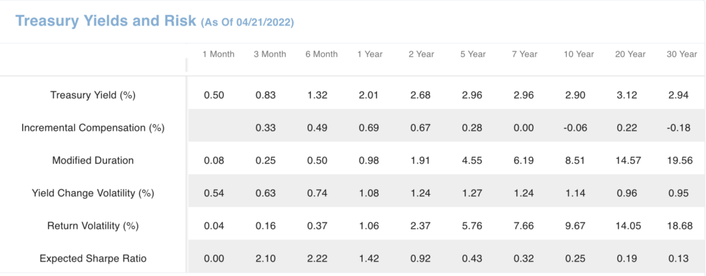
Modified Duration is a sensitivity measure of interest rate level (parallel shift) risk.
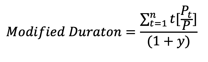
The numerator is Macaulay Duration. It is the time weighted (t =1,2, … n) present value of its cash flows where
is the present value of the cash flow at time t. P is the price of the bond and y is the yield to maturity. Alternatively, Macaulay Duration is the present value weighting of the timing of the cash flows. It is the return (change in price over prior price) sensitivity for a percentage change in yield. By dividing by (1+y), Modified Duration provides the more convenient return sensitivity to an absolute 1% change in yield,
Rate of Return = – ModifiedDuration * Change in Yield
A positive change in yield produces a bond price decline and a negative rate of return. A negative change in yield produces a bond price increase and a positive rate of return. Note that Modified Duration increases with maturity. Earlier coupons and principal payments can be reinvested at the new yields rather than be locked in for longer maturities.
Modified Duration provides the sensitivity to yield changes, but a measure of change in yield dispersion is required to obtain a measure of return volatility. Yield Change Volatility (standard deviation) is a measure of dispersion of yields around its average. Then, Return Volatility is the investment risk measure,
Return Volatility = ModifiedDuration * Yield Change Volatility
It combines the yield change volatility with the sensitivity to changes in yield (Modified Duration).
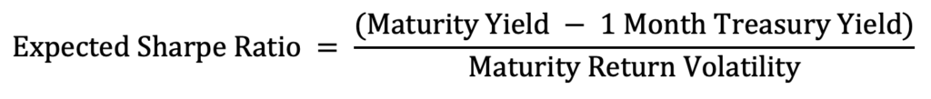
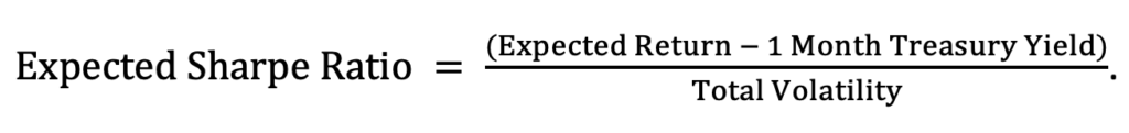
The Expected Sharpe Ratio provides a measure of expected risk-adjusted performance. It is the expected excess yield for a specific maturity less that of the 1 Month Yield per unit of its Return Volatility.
Note the highest expected excess yield per unit of return volatility is currently at 6 months. The incremental compensation drops off substantially after 2 years. That is consistent with the bulk of the maturity premium required to encourage investors to take on more interest risk is within 2 years. Given that the highest expected Sharpe ratio is at 6 months, hedge funds would rather leverage up (borrow at or near the one-month yield) and invest 20 times their capital on a 6-month Treasury than purchase a Treasury bond with 10 years of modified duration. Much more expected yield in the leveraged strategy for similar interest rate risk.
Furthermore, an investor that strongly believes interest rates will rise more than the market expects, may lower exposure to rate increases (declining bond prices) by lowering bond portfolio modified duration (less sensitivity). Likewise, an investor that strongly believes interest rates will decline more than the market expects, may increase exposure to interest rates falling (increasing bond prices) with higher bond portfolio modified duration (greater sensitivity).
The calculation of modified duration for US Treasury Bills, Notes and Bonds works well for small changes in interest rates. As rates change, modified duration should be recalculated.
The reason the calculation is easy and accurate for Treasury securities is that the timing and magnitude of all cash flows (principal and coupon interest payments) are known for certain. There is no default risk because Treasuries are backed by the full faith and credit of the US government with a money printing press and taxing authority to make all required payments.
Agency Mortgage-Backed Securities (MBS) also have no default risk, but the timing of receiving payments is uncertain. It depends on homeowner decisions on refinancing when mortgage rates decline below what they are currently paying, moving to another location for job opportunities or the inability to maintain payments. Whether it is from the homeowner refinancing or from government backed (Fannie Mae, Freddie Mac or Ginnie Mae) mortgages in default, the cash flows will come in sooner to MBS investors than its stated maturity. Mortgages also have a principal paydown in every monthly payment while Treasury and corporate bonds typically have the full principal paid at maturity.
Since cash flows are expected to come in much earlier than the 30-year MBS contract maturity, the interest rate risk of a newly originated pool of 30-year MBS is more like the interest rate sensitivity of a 10-year Treasury note than a 30-year Treasury bond.
Furthermore, after origination the expected prepayments over the remaining life of the mortgage pool is interest rate path dependent. For example, as rates decline, prepayments are expected to accelerate, moving cash flows earlier and lowering interest rate risk. If the mortgage origination rate declines substantially prepayments will occur on a large percentage of the pool. However, if the mortgage rate goes back up toward the origination rate (no prepayment incentive) and then goes back down to the previous low, prepayments will be much slower than the first time. That is because the credit impaired or oblivious borrower is now the bulk of the remaining pool. Those in the pool that were ready, willing, and able to refinance are gone. Both expected prepayments and duration are changing throughout the interest rate path as well.
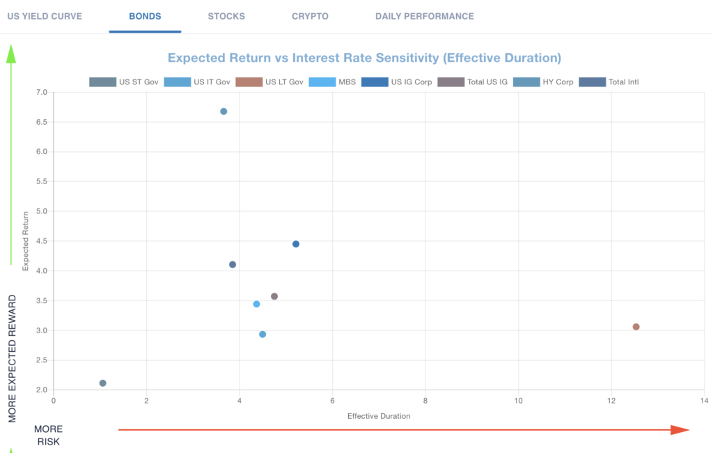
Therefore, using the modified duration formula for Treasuries would be a gross overestimation of interest rate sensitivity for risky bonds. Instead, Ripsaw® provides an empirical methodology that uses the information in prices for the time-varying changes in Effective Duration due to changes in the yield curve and risk premiums. This Effective Duration methodology is also used for corporate bonds since changes in the yield curve and stock return volatility also has implications for expected profitability (i.e., economic growth, recession) and the expected probability distribution of default. Default will move any remaining cash flow earlier and with less magnitude (recovery rate to lenders).
All bonds have degrees of interest rate risk approximated by Effective Duration. Government funds only have interest rate risk. Agency Mortgage-Backed Securities (MBS) also have prepayment risk. Corporate bonds also have default risk. The US IG (Investment Grade) fund contains Treasury, MBS and Corporate bonds with all three risk factors: interest rate, prepayment and default.
Models of an investment’s forward-looking expected return and risk requires unbundling the risk components of the investment and determining the market’s required compensation for bearing each risk. Having an accurate estimate of Effective Duration is essential for finding a Duration-Matched Treasury Yield as the interest rate risk match. For corporate bonds and MBS there are the additional systematic risks of default and the timing of prepayments, respectively, that require risk premiums as compensation.
The forward-looking Expected Return on each sector of the bond market is the sum of its duration-matched Treasury yield (compensation for interest rate risk) plus the Ripsaw® model of expected risk premium (compensation) for prepayment and default risks.
Expected Return = Duration Matched Treasury Yield + Risk Premium
Total Volatility (standard deviation) contains all risk dimensions in a fund investment.
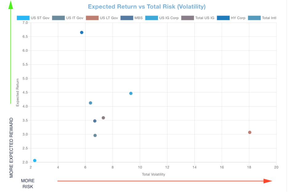
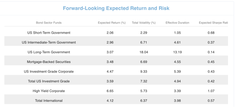
The Expected Sharpe Ratio provides a measure of expected risk-adjusted performance. It is the expected return for a fund less that of the 1 Month Treasury Yield per unit of its Total Volatility (Risk).
Currently, the high yield corporate bond sector has the highest Expected Sharpe Ratio. Its relatively low Effective Duration is consistent with more of Total Volatility coming from default risk. Its high expected return per unit of risk makes it a desirable part of a bond portfolio in isolation. However, this default risk is correlated with stock market risk. It is important to always be thinking about your entire cash, bond and stock portfolio risk and expected return. Diversification benefits are likely to have both sources represented in the right proportions in an investor’s total wealth portfolio optimization.
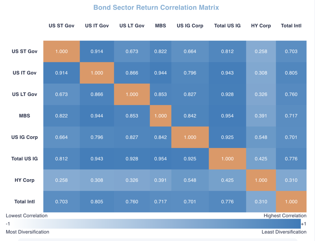
The Bond Return Correlation Matrix contains all pairwise return correlations between bond sector funds. The lower the correlation, the greater the benefit from diversification. The Government funds only have interest rate risk. Their correlations are high, but not perfect because we are only including interest rate level (parallel shift) risk proxied by changes in the 10-year Treasury rate. Interest rate level risk is the most explanatory component. The remaining smaller interest rate risks (i.e., slope and curvature) are not included at this time, but in development. Note the lowest correlations are between the High Yield Corporate sector and the others. That is because it has a low interest rate level risk contribution to total volatility and a high default (below Investment Grade) risk contribution that is not present in the other sector funds.
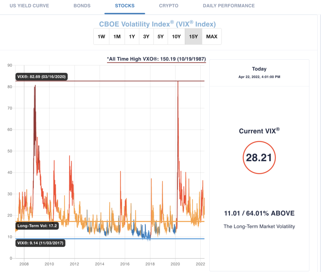
For the stock market, The CBOE Volatility Index®, or VIX®, is a real-time market index representing the market’s expectation for volatility over the coming 30 days (forward-looking). Investors use VIX® as a measure of the level of risk in the market when making investment decisions. The higher the current risk (VIX®), the greater the market risk premium investors require to have them hold the S&P 500 stock portfolio over the 1-month Treasury Bill, especially for short-term investment horizons. The lower the current market risk (VIX®), the lower the risk premium required by the market.
VIX® goes down, risk premium declines and S&P 500 portfolio value goes up. VIX® goes up, the risk premium increases, and S&P 500 portfolio value goes down. Sounds like a potential trading strategy. Yes and no. If you could accurately predict changes in VIX® over short intervals, the answer would be yes to a profitable trading strategy. Since large VIX® movements are primarily the result of surprises, it is unlikely that short-term trading strategies will generate consistent profits. However, VIX® does contains important information concerning the market’s current consensus view of future volatility and the risk premium reflected in prices. This is useful information that should be considered in tactical asset allocation decisions. For example, an extraordinary high VIX (substantially greater than historical average) reflects a much higher than average risk premium demanded by market participants in the short term.
These scenarios represent an opportunity for long-term investors to increase their stock allocation and then reduce that allocation back to their strategic stock allocation when VIX® returns to its long run average (resolution of temporary uncertainty). Short-term investors view stock market risk as current VIX® while long-term investors view their risk as long-term volatility. Essentially reaping the price increase associated with the reduction in risk premium. This strategy still carries the risk that the resolution of uncertainty is a good outcome (i.e., a tax cut) and not a bad outcome (i.e, a tax increase) for expected cash flows to shareholders. Moreover, a tactical increase in stock allocation when VIX® is currently at 28.21 (11 points or 64% above long-term volatility) may still go much higher generating losses on the tactical trade before the reversion to the mean (long-term average) occurs. Therefore, a layering in strategy can be implemented based on previous highs in VIX® and the all-time high on October 19, 1987. Do not get too far over your skis. Make sure your long-term investment horizon is sufficient for you to stay in the trade.
Similar tactical trading opportunities exist when VIX® is well below its long-run average. Tactically reducing a stock allocation when the compensation (risk premium) is low and waiting for a return to normal volatility will avoid losses before returning to a strategic asset allocation when the compensation is sufficient. It is also important to note the long periods of relatively low volatility requires the discipline of maintaining a low risk profile. Furthermore, VIX® can be an important tool in risk budgeting among asset classes.
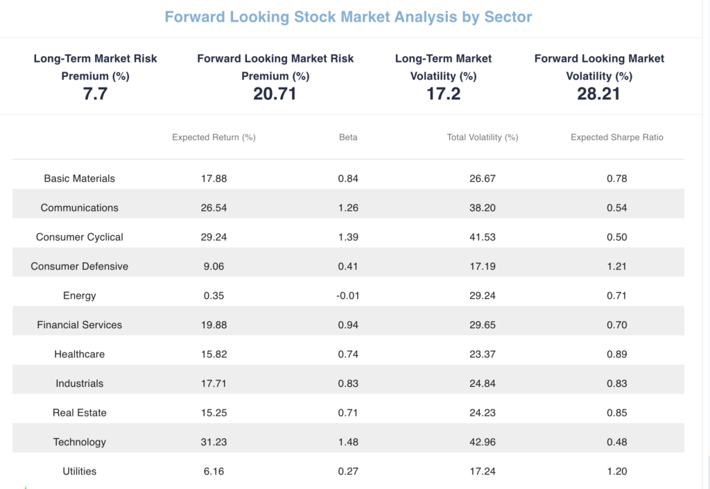
The long-term realized market risk premium of 7.7% is a reasonable estimate of what compensation, on average, the market required to hold the riskier S&P 500 stock portfolio versus the 1-month Treasury Bill. The incremental risk is the 17.2% long-term market volatility of the S&P 500 return. The 7.7% and 17.2% realized values for the Long-Term Market Risk Premium and Long-Term Market Volatility, respectively, are from the 49-year period (1972-2020) in Exhibit 2.14 on page 38 of the SBBI® 2021 Summary Edition.
To update for the current market risk premium associated with current VIX, Ripsaw® uses the relationship:

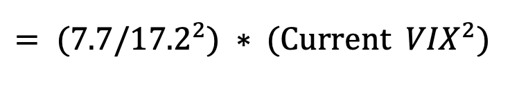
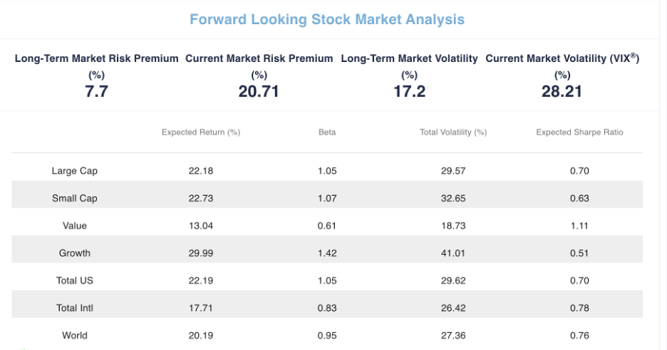 The forward-looking expected return on each stock fund is the current 1-month Treasury Bill yield plus the Fund’s Beta times the Current Stock Market Risk Premium. The Beta is an estimate of the fund’s return sensitivity to a stock market return.
Expected Return = Current1MonthTBillYield + [Beta*CurrentMarketRiskPremium]

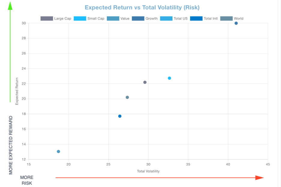
The forward-looking stock fund Total Return Volatility considers its two components: market returns and non-market returns. New macro information (i.e., changes in monetary policy, fiscal policy, economic growth, employment growth, global shocks) affect all securities, but to different degrees as represented by its Beta (sensitivity) to Market Return Volatility. Non-Market Return Volatility is associated with firm-specific risks (i.e., management capabilities, industry competitiveness, product life cycle). Ripsaw® employs econometric techniques to estimate Beta and solve for the Non-Market Volatility. The major source of changes in Total Return Volatility is from the changes in Market Return Volatility for which VIX® is the ideal update.

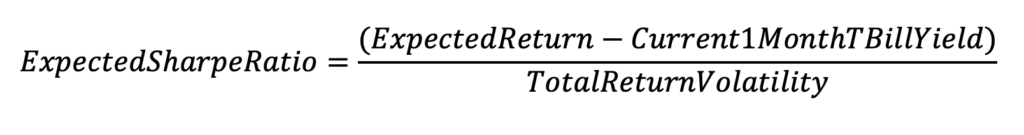
The forward-looking Expected Sharpe Ratio provides a measure of expected risk-adjusted performance. It is the expected return for the fund less that of the current 1-Month Treasury Yield per unit of the fund’s Total Return Volatility (Risk).
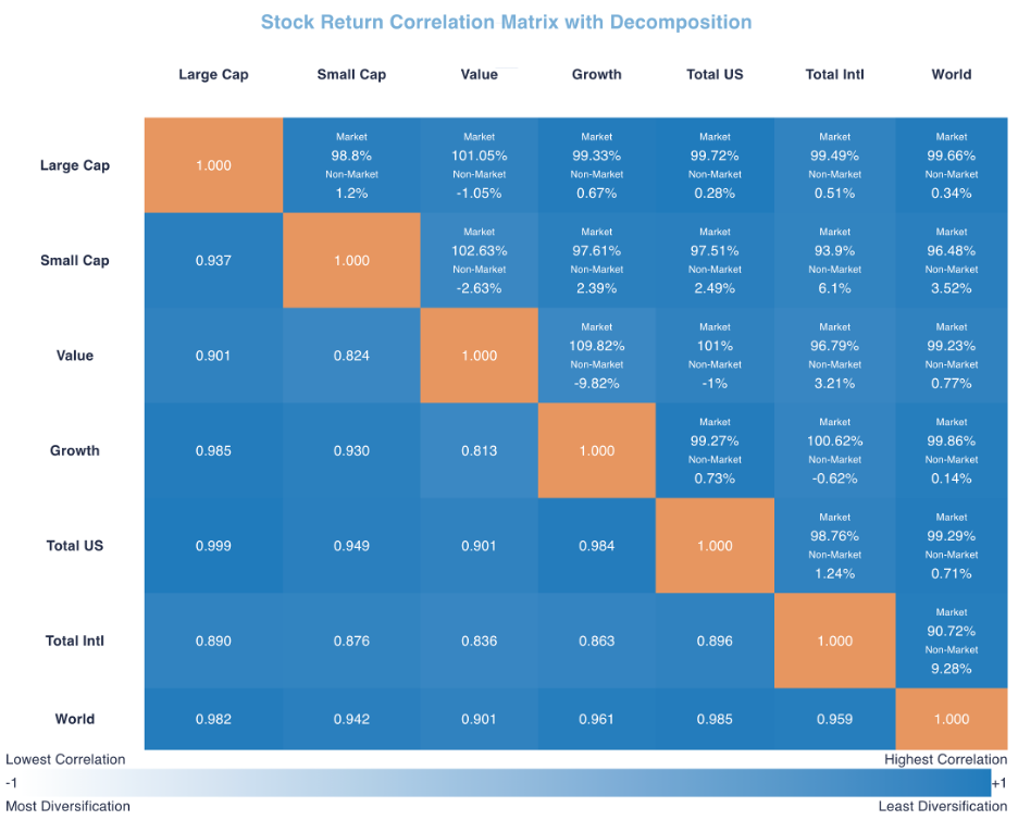
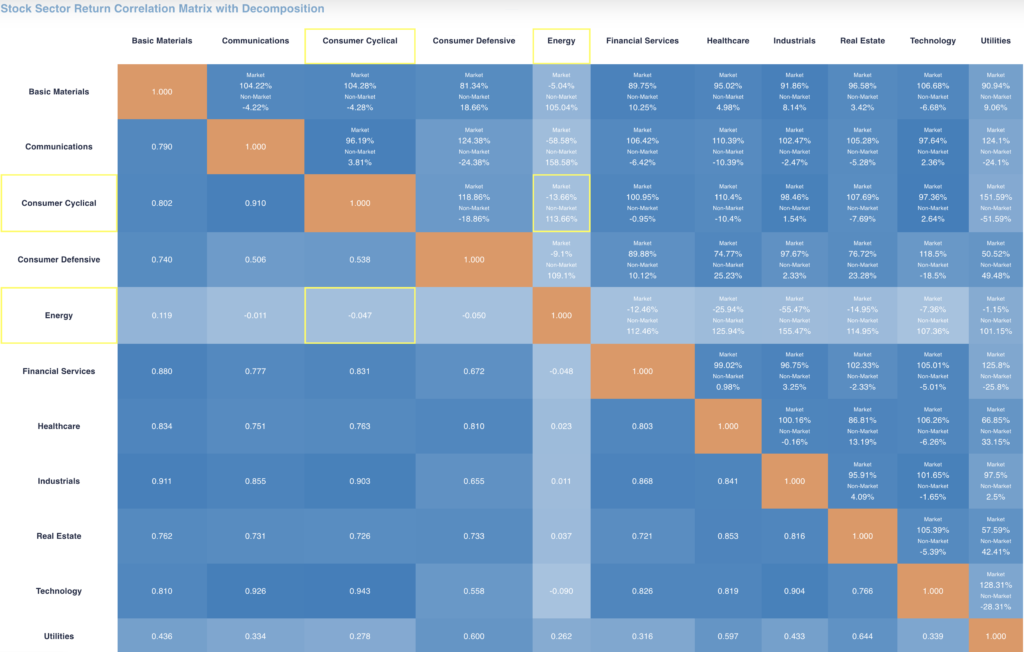
The forward-looking Stock Fund Correlation Matrix with Decomposition contains all pairwise return correlations between the stock funds. The lower the correlation, the greater the benefit from diversification.
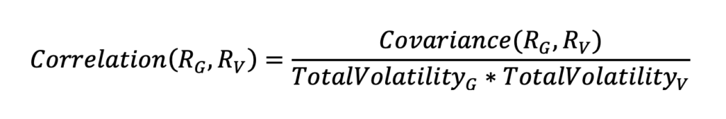
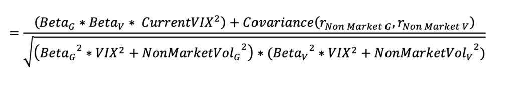
 For example, the pairwise return correlation between the Value and Growth funds is
Substituting the market and non-market breakdown including Current VIX® for the update on market volatility provides a forward-looking correlation,
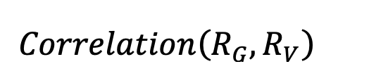
This methodology for an estimate of forward-looking correlation is also consistent with the frequently observed increase in all pairwise stock correlations as market volatility rises and a decrease in all pairwise stock correlations as market volatility declines. The market and non-market components have a percentage contribution to total correlation. These percentage contributions are in the right-hand-side triangle of the correlation matrix. Total correlation is in the left-hand-side triangle of the correlation matrix. In the future, as VIX increases, the market percentage contribution increases with no diversification benefit. The non-market percentage contribution that has a diversification benefit declines. That combination increases total correlations. As market volatility declines, the market percentage contribution declines and the non-market percentage contribution with its diversification benefit increases. That combination lowers total correlations. Substituting VIX for Market Volatility updates all known information for future market volatility assessment rather than wait for historical data estimates of market volatility to catch up.
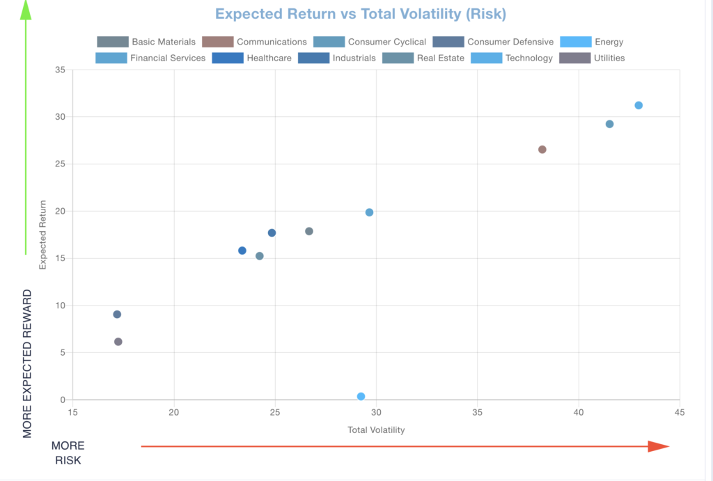
A diversified stock portfolio will have representation from all sector classifications in the market. The economy has just printed a -1.4% economic growth number for the first quarter of 2022. This may be the first leg of a recession (two consecutive quarters of negative economic growth). That is consistent with the Consumer Defensive and Utilities sectors having the highest Expected Sharpe Ratios due to substantially lower volatilities. The highest volatilities are in the Consumer Cyclical and Technology sectors implying their greater uncertainty in a declining economy.
In the Stock Sector Correlation Matrix with Decomposition, the Energy sector has extremely low correlation with all other sectors. An important component of inflation and its role in slowing the economy is the shortage of energy and the dramatic increase in value of that commodity. Note that its recent Beta is slightly negative, making its covariance through the market (systematic risk) negative as well as its negative non-market covariance. Negative beta and negative correlation with other sectors are major risk reducing investments.
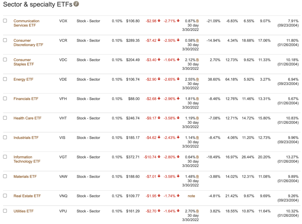
In the return section for each sector ETF provided by Vanguard (https://investor.vanguard.com/etf/list#/etf/asset-class/month-end-returns), the Year-To-Date (YTD) return on the Energy ETF was +38.6% while 8 sectors have negative returns and only 2 have small positive returns. The worst return of -21.09% was from the Communication Services ETF. Therefore, significantly underweighting the Energy sector implies poor portfolio diversification and substantial underperformance. In this case, it was the Energy sector underweight that had adverse consequences. In the future, any significant sector underweight could have unintended consequences. The lesson is to monitor portfolio stock sector composition and not stray too far from your benchmark composition. All this monitoring for your portfolio and its revision decisions are readily available in Ripsaw® Wealth Tools.

Try Ripsaw Market and the rest of Ripsaw® Wealth Tools today!!